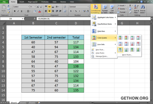
Microsoft excel is the branch of Microsoft Office, excel has the feature to calculate any longest account in there sheets in seconds of time. Here we have color conditional formatting rule in Microsoft excel application. First know that what color conditional format is actually, so it is a rule for the numeral values to show different colors for low mid and high rates of numbers in cells. Just like a place where stock exchange uses various colors to show the up going and down going shares rate in real time whenever basic value changes.
What you need first for conditional format
If you have already a ready made or self made excel file which have some calculation made within the file then you can go ahead for doing the conditional formats to the excel sheets value. You need a column line either one or many which depends on your data sheet which contains the output result of the entire calculation. Suppose if you have a result excel sheet of college which contains 3 columns of 1st semester, 2nd semester and total column so you have to use 3rd column that is total column for conditional formatting.
How to apply color conditional formats in excel
To apply the color based conditional formats just select the whole column except the title and just go to Home Tab and then click on conditional formatting under which click on Color Scales where you will have some of the color based formatting by default which appear on hover of mouse there. Click on any favorable color condition which you like and you are done.
[ Step : Select Any Output Column Without Title » Home Tab » Conditional Formatting » Color Scales » Select Any One Effect You Like ]
This is one small trick to use color based formatting in excel, however this feature is hugely used in companies and large scale organization up till now. Enjoy this color formatting in excel.

